Graphs
A processing pipeline in DALiuGE is described by a Directed Graph where the nodes denote both task (application DROPs) and data (data DROPs). The edges denote execution dependencies between DROPs. Section DALiuGE Functions has briefly introduced graph-based functions in DALiuGE. This section provides implementation details in the DALiuGE prototype.
Logical Graph
A logical graph is a compact representation of the logical operations in a processing pipeline without concerning underlying hardware resources. Such operations are referred to as construct in a logical graph. The relationship between a DROP and a construct resembles the one between and object and a class in Object Oriented programming languages. In other words, most constructs are DROP templates and multiple DROPs correspond to a single construct.
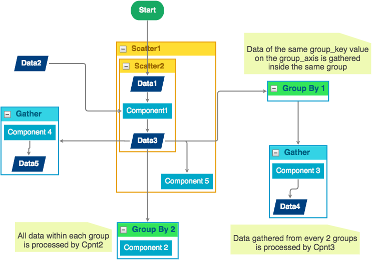
Fig. 2 An example of a logical graph with data constructs (e.g. Data1 - Data5), component constructs (i.e. Component1 - Component5), and control flow constructs (Scatter, Gather, and Group-By). This example can be viewed online in the DALiuGE prototype.
Construct properties
Each construct has several associated properties that users have control over during the development of a logical graph. For Component and Data constructs the Execution time and Data volume are two very important properties. Such properties can be directly obtained from parametric models or estimated from the profiling information (e.g. pipeline component workload characterisation) and COMP platform specification.
Control flow constructs
Control flow constructs form the “skeleton” of the logical graph, and determine the final structure of the physical graph to be generated. DALiuGE currently supports the following flow constructs:
Scatter indicates data parallelism. Constructs inside a Scatter construct represent a group of components consuming a single data partition within the enclosing Scatter. A useful property of Scatter is
num_of_copies. In the example in Fig. 2, if thenum_of_copiesforScatter1andScatter2are 5 and 4 respectively, the generated physical graph will have in total 20Data1/Component1/Data3DROPs, but only 5 DROPs for the constructComponent 5, which is inside theScatter1construct but outsideScatter2.Gather indicates data barriers. Constructs inside a Gather represent a group of components consuming a sequence of data partitions as a whole. Gather has a
num_of_inputsproperty, which represents the Gather “width”, stating how many partitions each Gather instance (translated into aBarrierAppDROP, see DROP Component Interface) can handle. This in turn is used by DALiuGE to determine how many Gather instances should be generated in the physical graph. Gather sometimes can be used in conjunction with Group By (see middle-right in Fig. 2), in which case, data held in a sequence of groups are processed together by components enclosed by Gather.Group By indicates data resorting (e.g. corner turning in radio astronomy). The semantic is analogous to the
GROUP BYconstruct used in SQL statement for relational databases, but applied to data DROPs. The current DALiuGE prototype requires that Group By is used in conjunction with a nested Scatter such that data DROPs that are originally sorted in the order of[outer_partition_id][inner_partition_id]are resorted as[inner_partition_id][outer_partition_id]. In terms of parallelism, Group By is comparable to the “static” MapReduce, where the keys used by all Reducers are known a priori.Loop indicates iterations. Constructs inside a Loop represent a group of components and data that will be repeatedly executed / produced for a fixed number of times. Given the basic DROP principle of “writing once, read many times”, the current DALiuGE prototype does not support dynamic branch condition for Loop. Instead, each Loop construct has a property named
num_of_iterationsthat must be determined at logical graph development time, and that determines the number of times the loop is “unrolled”. In other words, anum_of_iterationsnumber of DROPs for each construct inside a Loop will be statically generated in the physical graph. An example is shown in Fig. 3.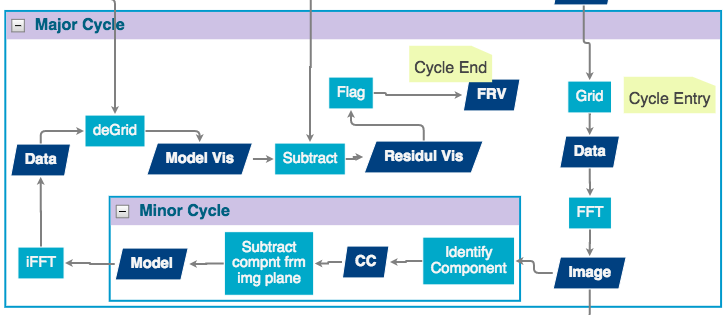
Fig. 3 A nested-Loop (minor and major cycle) example of logical graph for a continuous imaging pipeline. This example can be viewed online in the DALiuGE prototype.
Repository
The DALiuGE prototype uses a Web-based logical graph editor as the default user interface to the underlying logical graph repository, which currently is simply a managed POSIX file system directory. Each logical graph is physically stored as a JSON-formatted textual file, and can be accessed and modified remotely through the logical graph editor via the RESTful interface. For example, the JSON file for the continuous imaging pipeline as shown partially in Fig. 3 can be accessed through HTTP GET. The editor also provides a Web-based JSON editor so that users can directly change the graph JSON content inside the repository.
Select template
While the DALiuGE logical graph editor does not differentiate between logical graph and logical graph template, users can create either of them using the editor (after all, the only differences between these two are the populated values for some parameters). Once a template is created or selected, users can simply copy and paste the JSON content into the new logical graph and fill in those parameter values (as construct properties) using the editor. Note that the public version of the logical graph editor has not yet opened its “create new logical graph” API.
Translation
While a logical graph provides a compact way to express complex processing logic, it contains high level control flow specifications that are not directly usable by the underlying graph execution engine and DROP managers. To achieve that, logical graphs are translated into physical graphs. The translation process essentially creates all DROPs and is implemented in the dlg.dropmake module.
Basic steps
DropMake in the DALiuGE prototype involves the following steps:
- Validity checking. Checks whether the logical graph is ready to be translated. This step is similar to semantic error checking used in compilers. For example, DALiuGE currently does not allow any cycles in the logical graph. Another example is that Gather can be placed only after a Group By or a Data construct as shown in Fig. 2. Any validity errors will be displayed as exceptions on the logical graph editor.
- Construct unrolling. Unrolls the logical graph by (1) creating all necessary DROPs (including “artifact” DROPs that do not appear in the original logical graph), and (2) establishing directed edges amongst all newly generated DROPs. This step produces the Physical Graph Template.
- Graph partitioning. Decomposes the Physical Graph Template into a set of logical partitions (a.k.a. DropIsland) and generates an order of DROP execution sequence within each partition such that certain performance requirements (e.g. total completion time, total data movement, etc.) are met under given constraints (e.g. resource footprint). An important assumption is that the cost of moving data within the same partition is far less than that between two different partitions. This step produces the Physical Graph Template Partition.
- Resource mapping. Maps each logical partition onto a given set of resources in certain optimal ways (load balancing, etc.). Concretely, each DROP is assigned a physical resource id (such as IP address, hostname, etc.). This step requires near real-time resource usage information from the COMP platform or the Local Monitor & Control (LMC). It also needs DROP managers to coordinate the DROP deployment. In some cases, this mapping step is merged with the previous Graph partitioning step to directly map DROPs to resources. This step produces the Physical Graph.
Under the assumption of uniform resources (e.g. each node has identical capabilities), graph partitioning is equivalent to resource mapping since mapping involves simple round-robin all available resources. In this case, graph partitioning algorithms (e.g. METIS [5]) actually support multi-constraints load balancing so that both CPU load and memory usage on each node is roughly similar.
For heterogeneous resources, which DALiuGE has not yet supported, usually the graph partitioning is first performed, and then resource mapping refers to the assignment of partitions to different resources based on demands and capabilities using graph / tree-matching algorithms[16] . However, it is also possible that the graph partitioning algorithm directly produces a set of unbalanced partitions “tailored” for those available heterogeneous resources.
In the following context, we use the term Scheduling to refer to the combination of both Graph partitioning and Resource mapping.
Algorithms
Scheduling an Acyclic Directed Graph (DAG) that involves graph partitioning and resource mapping as stated in Basic steps is known to be an NP-hard problem. The DALiuGE prototype has tailored several heuristics-based algorithms from previous research on DAG scheduling and graph partitioning to perform these two steps. These algorithms are currently configured by DALiuGE to utilise uniform hardware resources. Support for heterogenous resources using the List scheduling algorithm will be made available shortly. With these algorithms, the DALiuGE prototype currently attempts to address the following translation problems:
- Minimise the total cost of data movement but subject to a given degree of load balancing. In this problem, a number N of available resource units (e.g. a number of compute nodes) are given, the translation process aims to produce M DropIslands (M <= N) from the physical graph template such that (1) the total volume of data traveling between two distinct DropIslands is minimised, and (2) the workload variations measured in aggregated execution time (DROP property) between a pair of DropIslands is less than a given percentage p %. To solve this problem, graph partitioning and resource mapping steps are merged into one.
- Minimise the total completion time but subject to a given degree of parallelism (DoP) (e.g. number of cores per node) that each DropIsland is allowed to take advantage of. In the first version of this problem, no information regarding resources is given. DALiuGE simply strives to come up with the optimal number of DropIslands such that (1) the total completion time of the pipeline (which depends on both execution time and the cost of data movement on the graph critical path) is minimised, and (2) the maximum degree of parallelism within each DropIsland is never greater than the given DoP. In the second version of this problem, a number of resources of identical performance capability are also given in addition to the DoP. This practical problem is a natural extension of version 1, and is solved in DALiuGE by using the “two-phase” method.
- Minimise the number of DropIslands but subject to (1) a given completion time deadline, and (2) a given DoP (e.g. number of cores per node) that each DropIsland is allowed to take advantage of. In this problem, both completion time and resource footprint become the minimisation goals. The motivation of this problem is clear. In an scenario where two different schedules can complete the processing pipeline within, say, 5 minutes, the schedule that consumes less resources is preferred. Since a DropIsland is mapped onto resources, and its capacity is already constrained by a given DoP, the number of DropIslands is proportional to the amount of resources needed. Consequently, schedules that require less number of DropIslands are superior. Inspired by the hardware/software co-design method in embedded systems design, DALiuGE uses a “look-ahead” strategy at each optimisation step to adaptively choose from two conflicting objective functions (deadline or resource) for local optimisation, which is more likely to lead to the global optimum than greedy strategies.
Physical Graph
The Translation process produces the physical graph specification, which, once deployed and instantiated “live”, becomes the physical graph, a collection of inter-connected DROPs in a distributed execution plan across multiple resource units. The nodes of a physical graph are DROPs representing either data or applications. The two DROP nodes connected by an edge always have different types from each other. This establishes a set of reciprocal relationships between DROPs:
- A data DROP is the input of an application DROP; on the other hand the application is a consumer of the data DROP.
- Likewise, a data DROP can be a streaming input of an application DROP (see Relationships) in which case the application is seen as a streaming consumer from the data DROP’s point of view.
- Finally, a data DROP can be the output of an application DROP, in which case the application is the producer of the data DROP.
Physical graph specifications are the final (and only) graph products that will be submitted to the DROP Managers. Once DROP managers accept a physical graph specification, it is their responsibility to create and deploy DROP instances on their managed resources as prescribed in the physical graph specification such as partitioning information (produced during the Translation) that allows different managers to distribute graph partitions (i.e. DropIslands) across different nodes and Data Islands by setting up proper DROP Channels. The fact that physical graphs are made of DROPs means that they describe exactly what an Execution consists of. In this sense, the physical graph is the graph execution engine.
In addition to DROP managers, the DALiuGE prototype also includes a Physical Graph Manager, which allows users to manage all currently running and past physical graphs within the system. Although the current Physical Graph Manager implementation only supports to “add” and “get” physical graph specifications, features such as graph event monitoring (through the DROP Events subscription mechanism) and the graph statistics dashboard will be added in the near future.
Execution
A physical graph has the ability to advance its own execution. This is internally implemented via the DROP event mechanism as follows:
- Once a data DROP moves to the COMPLETED state it will fire an event
to all its consumers. Consumers (applications) will then deem if they can start their
execution depending on their nature and configuration. A specific type of
application is the
BarrierAppDROP, which waits until all its inputs are in the COMPLETED state to start its execution. - On the other hand, data DROPs receive an even every time their producers finish their execution. Once all the producers of a DROP have finished, the DROP moves itself to the COMPLETED state, notifying its consumers, and so on.
Failures on applications and data DROPs are transmitted likewise automatically via events. Data DROPs move to ERROR if any of its producers move to ERROR, and application DROPs move the ERROR if a given input error threshold (defaults to 0) is passed (i.e., when more than a given percentage of inputs move to ERROR) or if their execution fails. This way whole branches of execution might fail, but after reaching a gathering point the execution might still resume if enough inputs are present.