Using the Logical Graph Editor
These are some guidelines on how to use the Logical Graph Editor included in DALiuGE.
General
On the left-hand side is the palette where different component types are shown. Users can drag these components and drop them in the central area where a Logical Graph will be build up. When hovering the mouse over a component on the Logical Graph different connection points appear on the borders of the component. By clicking on these and dragging the mouse over to a different component users can draw an arrow between two components signaling a relationship between the two.
By clicking on a component’s text users can also change the label shown by that component on the Logical Graph. This is useful for readability and has no impact on the final output of the Logical Graph.
Also when clicking on a component the editor will show the component’s properties on the bottom-right corner. Users can change here some values associated to the components. Different components support different properties.
Components
ShellApp
The ShellApp component represents a bash shell command.
The command to be run is written using
its different Arg properties.
For example, to run echo 123
users would have to write echo in Arg01
and 123 in Arg02.
When referring to the application’s inputs and outputs
in the command line
%i[X] and %o[X] can be used, respectively,
where X refers to the key property
of the referenced input/output.
These placeholders will eventually be replaced
with the file path of the corresponding inputs or outputs
when executing the command.
For inputs and outputs that are not filesystem-based
the %iDataURL[X] and %oDataURL[X] placeholders
can be used instead.
Note that sometimes an application is connected
to an input or output component
representing more than one physical input or output
(e.g., an application outside a Scatter component
connected to a Data component inside the Scatter).
In these cases the corresponding placeholder will expand
to a semicolon-delimited list of paths or URLs.
It will be the responsibility of the application
to deal with these cases.
Data
The Data component represents a payload.
When transitioning from the Logical Graph to the Physical Graph
these components generate InMemory drops currently,
but support will be added in the future
to generate drops with different storage mechanisms.
Scatter
The Scatter component represents parallel branches of execution.
Is is represented by a yellow-bordered box
that allows other components to be placed within.
All the contents of the body of a Scatter
will be replicated as parallel branches of execution
when performing the Logical Graph to Physical Graph transition
depending on the value of its num_of_copies property.
Components outside a Scatter
can be connected to components inside the Scatter.
In such cases, when he Physical Graph is generated,
the outside component will appear as connected
to the many copies generated from inside the Scatter.
Examples
Simple scatter
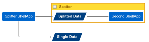
In this example we will have an application producing many outputs, identical in nature, which are then processed in parallel by a second application. The initial application also outputs a different, single file.
To do this we drop a ShellApp into the Logical Graph.
Next to it we drop a Scatter component.
Inside the Scatter component we drop a Data component,
and next to the Data component we finally drop
a second ShellApp component.
One can then draw an arrow
from the first ShellApp to the Data component,
and a second one
from the Data component to the second ShellApp.
Finally, drop a Data component outside the Scatter
and draw an arrow from the first ShellApp component into it.
Optionally change the names of the components
for readability.
The final result should look like this:
If you save the Logical Graph form above, and then generate the Physical Graph it will look like this:
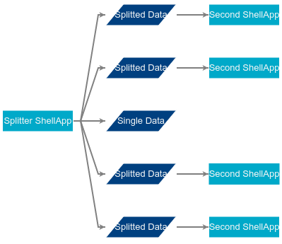
Here it can be clearly seen
how the Scatter component’s body
has been replicated according to its configuration.
It also shows how the first application
now produces multiple outputs.