Graphs
A processing pipeline or workflow in DALiuGE is described by a Directed Graph where the nodes denote both task (application components) and data (data components). The edges denote execution dependencies between components. Section Operational Concepts has introduced graph-based functions in DALiuGE. This section provides a more detailed overview of the internals of DALiuGE graphs.
Logical Graph
A logical graph is a compact representation of the logical operations and data flow in a processing workflow without being concerned about the underlying hardware resources. Logical graphs are constructed by domain experts who have a clear idea about the steps required to generate the desired science prducts. Many of the components are very domain specific and there are a number of different radio astronomy application and data components available to design logical graphs representing radio astronomy workflows. In addition to simple components DALiuGE also provides a number of complex components to support the encoding of higher level language operations like loop, scatter, gather and group-by. In particular the scatter complex component allows users to encode possible paralellisation of operations and whole sections of the graph. It should be noted though, whether those parts are really executed in parallel or serial depends on the actual deployment and availability of resources capable of the desired parallelism. Such complex components are also referred to as constructs in a logical graph. Constructs are not domain specific, but internally they do refer to simple components, which in turn might be domain specific. For instance a scatter construct might need a very domain specific way of splitting up and preparing the data for every single branch of the scatter.
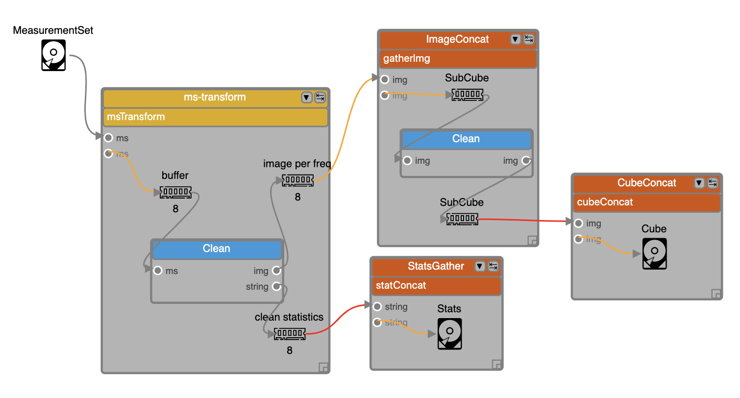
Fig. 1 An example of a logical graph with various types of data components as well as simple and complex application components. The graph uses two types of data components, File and Memory, depicted by respective icons. The titles shown with the icons, e.g. MeasurementSet, buffer, SubCube and Stats, refer to the actual content of those data components. There are two simple application components used in this graph, both are refering to the same application called Clean. In addition there are four complex components, one scatter construct (ms-transform) and three gather constructs (ImageConcat, CubeConcat and StatsGather). This example can be viewed online in EAGLE. (Note: this requires that you have setup EAGLE with a valid gitHUB access token, see EAGLE help)
Logical Graphs will be translated into physical graphs and at that point the component descriptions will be turned into Drop descriptions (see Drops). At execution time these Drop descriptions will be instantiated by the execution engine managers.
Component properties
Each component has several associated parameters that users have control over during the development of a logical graph. For Application and Data components the Execution time and Data volume are two important parameters. These properties can be directly obtained from parametric models or estimated from profiling information (e.g. pipeline component workload characterisation) and information about the hardware capabilities.
Complex components (Constructs)
Constructs form the “skeleton” of the logical graph, and determine the final structure of the physical graph to be generated. DALiuGE currently supports the following flow constructs:
Scatter indicates data parallelism. The group of components inside a Scatter construct are consuming a single data partition within the enclosing Scatter. The most important user defineable parameter of Scatter is
Number of Splits. In the example in Fig. 1, if theNumber of SplitsforScatter1andScatter2are 5 and 4 respectively, the generated physical graph will have in total 20Data1/Component1/Data3Drops, but only 5 Drops for the constructComponent 5, which is inside theScatter1construct but outsideScatter2.Gather indicates data barriers. Constructs inside a Gather represent a group of components consuming a sequence of data partitions as a whole. Gather has a
Number of Inputsproperty, which represents the Gather “width”, stating how many partitions each Gather instance (translated into aBarrierAppDROP, see Drop Component Interface) can handle. This in turn is used by DALiuGE to determine how many Gather instances should be generated in the physical graph. Gather sometimes can be used in conjunction with Group By (see middle-right in Fig. 1), in which case, data held in a sequence of groups are processed together by components enclosed by Gather. NOTE: The flexibility of Scatter and Gather constructs allow users to design complex data flow graph patterns by just changing theNumber of SplitsandNumber of Inputsparameter. However, changing those seemingly simple values may lead to unexpected or even wrong physical graphs. Users should thus always verify the _pattern_ of the constructed physical graphs on a small but representative scale.Group By indicates data resorting (e.g. corner turning in radio astronomy). The semantic is analogous to the
GROUP BYconstruct used in SQL statement for relational databases, but applied to data Drops. DALiuGE requires that Group By is used in conjunction with a nested Scatter such that data Drops that are originally sorted in the order of[outer_partition_id][inner_partition_id]are resorted as[inner_partition_id][outer_partition_id]. In terms of parallelism, Group By is comparable to the “static” MapReduce, where the keys used by all Reducers are known a priori. NOTE: As with the Scatter and Gather constructs, Group By constructs provide a very powerful way to change the structure of reduction graphs. Users are advised to always check the resulting physical graph _patterns_ for correctness.Loop indicates iterations. Constructs inside a Loop represent a group of components that will be repeatedly executed for a fixed number of times. Although there is also a Branch construct, the current DALiuGE implementation does not support dynamic branch conditions inside a Loop. Instead, each Loop construct has a property named
Number of Iterationsthat must be determined at logical graph development time, and that determines the number of times the loop is “unrolled”. In other words, aNumber of Iterationsnumber of Drops for each construct inside a Loop will be statically generated in the physical graph. An example is shown in Fig. 2.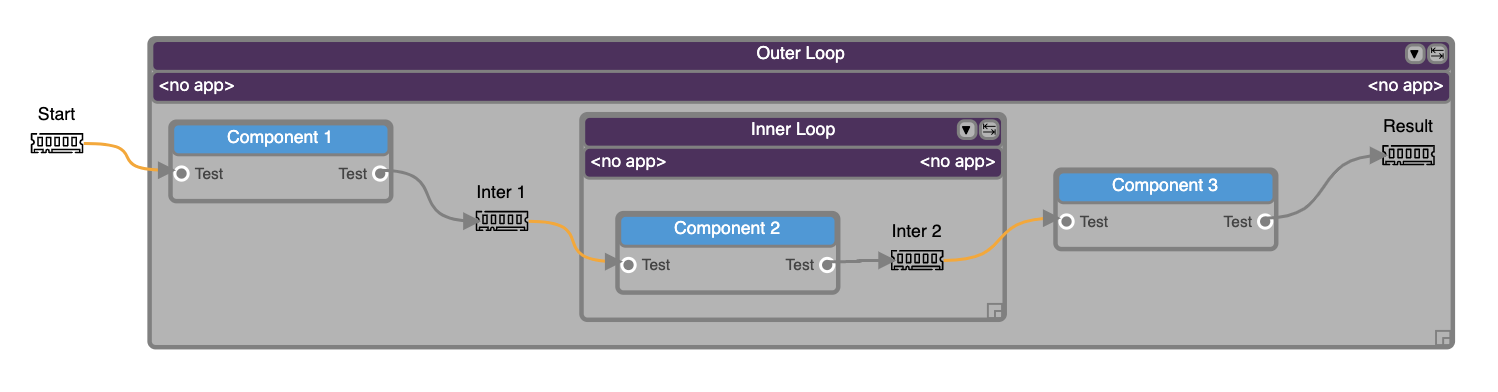
Fig. 2 A nested-Loop (outer and inner) example of logical graph for a continuous imaging pipeline. This example can be viewed online in DALiuGE.
Branch indicates conditional execution of sections of a physical graph. Branching (as well as loops) are, maybe surprisingly, tricky cases to deal with in a dataflow and DAG environment. Both of them are either explicitly (loop) or potentially (branch) producing cycles and are thus not directly representable as a DAG and thus it is hard to construct a physical graph. Branch constructs have the additional issue that one side of the branch, depending on the condition, might never be executed. Since the condition result in general is only known at runtime, the physical graph that will actually be executed can’t be computed upfront and thus scheduling as well as resource planning can only be done as an upper (or lower) limit. Although branches do work in DALiuGE, currently in most of the cases the graph execution will not finish, since the engine can’t discard whole physical graph sections based on a runtime condition and thus the graph will never reach the FINISHED state. We will tackle this issue in a future release.
MKN generalised scatter/gather. While designing the Scatter, Gather and Group By constructs we have found that it is possible to generalise these constructs into what we called MKN construct. MKN stands for a multiplicity of M externally to the construct, K internal and N on the output side. The MKN constructs are not fully supported throughout the DALiuGE framework yet, but will provide even more powerful ways to construct complex graph patterns. The current implementation is limited to what Scatter and Gather constructs are doing and thus using those is equivalent and the preferred solution for now.
Repositories
DALiuGE uses EAGLE, a Web-based logical graph editor as the default user interface to underlying logical graph and component repositories. Repositories can reside on a local file system, on GitHub or on GitLab. Each logical graph is physically stored in those repositories as a JSON-formatted text file. The JSON format is based on a JSON schema and validated against that as well. The JSON file contains the description of the application and data components used in the graph as nodes, a description of the connection between the nodes (edges and connection ports) and also the description of some of the representation properties required to draw the graph.
The repositories also contain so-called palettes, which represent a collection of components. Users can pick from those components in EAGLE to draw logical graph templates. The differentiation between graphs and palettes is somewhat blurry, since any graph can also be used as a collection of components. However, palettes usually contain a superset of components used in any graph derived from them and thus the distinction is still relevant.
Usage of Logical Graph Templates and Logical Graphs
EAGLE currently does not explicitely differentiate between a logical graph and a logical graph template. The only difference between these two are the populated values for some parameters and the relationship between the two is similar to the relationship between classes and instances in an OO language. The graphs in the repositories in general are logical graph templates (i.e. classes). The Users can simply load a logical graph from one of the repositories and modify the existing parameters before submitting to the translator. In future we will extend the repository functionality of EAGLE to deal with logical graphs and logical graph templates and also bind the logical graphs to execution sessions in the DALiuGE engine.
Translation
While a logical graph provides a compact way to express complex processing logic, the complex components or constructs are not directly usable by the underlying graph execution engine and Drop managers. To achieve that, logical graphs are translated into physical graphs. The translation process makes the parallelism explicit and unrolls loops and creates all Drop descriptions. Drops are essentially instances of the components. It is implemented in the dlg.dropmake module.
Basic steps
DropMake in DALiuGE involves the following steps:
Validity checking. Checks whether the logical graph is ready to be translated. This step is similar to semantic error checking used in compilers. For example, DALiuGE currently does not allow any cycles in the logical graph. Another example is that Gather can be placed only after a Group By or a Data component as shown in Fig. 1. Validity errors will be displayed as exceptions on the logical graph editor.
Construct unrolling. Unrolls the logical graph by (1) creating all necessary Drops (including “artifact” Drops that do not appear in the original logical graph), and (2) establishing directed edges amongst all newly generated Drops. This step produces the physical graph template.
Graph partitioning. Decomposes the Physical Graph Template into a set of logical partitions (a.k.a. DataIsland) and generates an order of Drop execution sequence within each partition such that certain performance requirements (e.g. total completion time, total data movement, etc.) are met under given constraints (e.g. resource footprint). An important assumption is that the cost of moving data within the same partition is far less than that between two different partitions. This step produces the Physical Graph Template Partition.
Resource mapping. Maps each logical partition onto a given set of resources in certain optimal ways (load balancing, etc.). Concretely, each Drop is assigned a physical resource id (such as IP address, hostname, etc.). This step requires near real-time resource usage information from the computing platform. It also needs Drop managers to coordinate the Drop deployment. In some cases, this mapping step is merged with the previous Graph partitioning step to directly map Drops to resources. This step produces the physical graph.
DALiuGE supports multiple algorithms implementing the latter two steps and users can choose between them when submitting the logical graph to the translator. Under the assumption of uniform resources (e.g. each node has identical capabilities), graph partitioning is equivalent to resource mapping since mapping could simply be implemented as a round-robin allocation to all available resources. For uniform resources, graph partitioning algorithms like e.g. METIS [5] actually support multi-constraints load balancing so that both CPU load and memory usage on each node is roughly similar.
For heterogeneous resources, which DALiuGE does not support yet, usually the graph partitioning is first performed, and then resource mapping refers to the assignment of partitions to different resources based on demands and capabilities using graph / tree-matching algorithms[16] . However, it is also possible that the graph partitioning algorithm directly produces a set of unbalanced partitions “tailored” for those available heterogeneous resources.
In the following context, we use the term Scheduling to refer to the combination of both Graph partitioning and Resource mapping.
Scheduling Algorithms
Optimally scheduling an Acyclic Directed Graph (DAG) that involves graph partitioning and resource mapping as stated in Basic steps is known to be an NP-hard problem. DALiuGE has tailored several heuristics-based algorithms from previous research on DAG scheduling and graph partitioning to perform these two steps. These algorithms are currently configured by DALiuGE to utilise uniform hardware resources. Support for heterogenous resources using the list scheduling algorithm will be implemented in a later release. With these algorithms, DALiuGE currently attempts to address the following optimisation goals:
Minimise the total cost of data movement but subject to a given degree of load balancing. In this problem, a number N of available resource units (e.g. a number of compute nodes) are given, the translation process aims to produce M DataIslands (M <= N) from the physical graph template such that (1) the total volume of data traveling between two distinct DataIslands is minimised, and (2) the workload variations measured in aggregated execution time (Drop property) between a pair of DataIslands is less than a given percentage p %. To solve this problem, graph partitioning and resource mapping steps are merged into one.
Minimise the total completion time but subject to a given degree of parallelism (DoP) (e.g. number of cores per node) that each DataIsland is allowed to take advantage of. In the first version of this problem, no information regarding resources is given. DALiuGE simply strives to come up with the optimal number of DataIslands such that (1) the total completion time of the pipeline (which depends on both execution time and the cost of data movement on the graph critical path) is minimised, and (2) the maximum degree of parallelism within each DataIsland is never greater than the given DoP. In the second version of this problem, a number of resources of identical performance capability are also given in addition to the DoP. This practical problem is a natural extension of version 1, and is solved in DALiuGE by using the “two-phase” method.
Minimise the number of DataIslands but subject to (1) a given completion time deadline, and (2) a given DoP (e.g. number of cores per node) that each DataIsland is allowed to take advantage of. In this problem, both completion time and resource footprint become the minimisation goals. The motivation of this problem is clear. In an scenario where two different schedules can complete the processing pipelinewithin, say, 5 minutes, the schedule that consumes less resources is preferred. Since a DataIsland is mapped onto resources, and its capacity is already constrained by a given DoP, the number of DataIslands is proportional to the amount of resources needed. Consequently, schedules that require less number of DataIslands are superior. Inspired by the hardware/software co-design method in embedded systems design, DALiuGE uses a “look-ahead” strategy at each optimisation step to adaptively choose from two conflicting objective functions (deadline or resource) for local optimisation, which is more likely to lead to the global optimum than greedy strategies.
In addition to the automatic deployment and scheduling options, there is also a special construct component available, called ‘Exclusive Force Node’, to allow users to enforce the placement of certain parts of the graph on a single compute node (NOTE: This is still work-in-progress.). In the case that a scattered section of the graph is enclosed in such an Exclusive Force Node construct, each of the scattered sections will be deployed on a compute node. In case there are not enough compute nodes available to accommodate all the scattered sections, some of them might be deployed (in whole, but together) on a single node. This also shows the risk of using such ‘hints’: It essentially reduces the degrees of freedom of the scheduling algorithm(s) and thus might turn out to be less optimal at runtime.
Physical Graph
The Translation process produces the physical graph, which, once deployed and instantiated on the DALiuGE execution engine, becomes a collection of inter-connected Drops in a distributed execution plan across multiple resource units, which we refer to as a physical graph Instance. The nodes of a physical graph Instance are Drops representing either data or applications, which represent the two base types of Drops. Any two Drops connected by an edge must have different base types, i.e. Drops along a physical graph Instance will have alternating base types. This establishes a set of reciprocal relationships between Drops:
A data Drop is the input of an application Drop; on the other hand the application is a consumer of the data Drop.
Likewise, a data Drop can be the output of an application Drop, in which case the application is the producer of the data Drop.
Similarly, a data Drop can be a streaming input of an application Drop (see Relationships) in which case the application is seen as a streaming consumer from the data Drop’s point of view.
Physical Graphs are the final (and only) graph products that will be submitted to the Drop Managers. Once Drop managers accept a physical graph, it is their responsibility to instantiate and deploy Drop instances on their managed resources as prescribed in the physical graph such as partitioning information (produced during the Translation) that allows different managers to distribute graph partitions (i.e. DataIslands) across different nodes by setting up proper Drop Channels. Once this instantiation phase is finished, the network of Drops and Drop channels is an exact representation of the physical graph and only needs an initial trigger to execute autonomously in a Execution. In this sense, the physical graph Instance is the actual graph execution engine, the managers are only required to instantiate the physical graph and send a trigger event to the start Drop. During execution the managers listen to Drop events and can in turn be used to monitor the execution progress. In order to facilitate the monitoring the Drop Managers also provide web interfaces as well as REST interfaces.
Execution
One of the unique features of DALiuGE is the complete decentralisation of the execution. A Physical Graph Instance has the ability to advance its own execution. This is internally implemented via the Drop event mechanism as follows:
Once a data Drop moves to the COMPLETED state it will fire an event to all its consumers. Consumers (applications) will then assert if they can start their execution depending on their nature and configuration. A specific type of application is the
BarrierAppDROP, which waits until all its inputs are in the COMPLETED state to start its execution.On the other hand, data Drops receive an event every time their producers finish their execution. Once all the producers of a Drop have finished, the Drop moves itself to the COMPLETED state, notifying its consumers, and so on.
Failures on applications and data Drops are transmitted likewise automatically via events. Data Drops move to ERROR if any of its producers move to ERROR, and application Drops move the ERROR if a given input error threshold (defaults to 0) is passed (i.e., when more than a given percentage of inputs move to ERROR) or if their execution fails. This way whole branches of execution might fail, but after reaching a gathering point the execution might still resume if enough inputs are present.
Parallelism
Speaking about execution, DALiuGE also exhibits multiprocessing of drops using Python’s native
multiprocessing library.
If enabled, drops are launched for execution on their own threads and all memory-drops become
shared-memory-drops which write to /dev/shm. While relatively robust, one should be careful
to ensure safe-access to memory-drops in this case, opting to use scatter/gather or other explicit
aggregation stages where necessary.